Project Gutenberg and Word2Vec

tl;dr I clustered top classics from Project Gutenberg using word2vec, here are the results and the code.

I had been reading up on deep learning and NLP recently, and I found the idea and results behind word2vec very interesting. word2vec is a technique to learn vector representations of individual words (called word vectors) by training over a large enough document or corpora. Although, I should mention word2vec is a shallow model, and shouldn’t be categorised as deep learning.

It learns by using words in the “context” of a target word to predict the occurrence of that word. The “context” is usually taken to be the surrounding words in a fixed size window on either side of the given word. These word vectors are then learned by training over all possible (context, target) pairs from the document or corpora.

The intricacies of the word2vec learning process are very interesting, and I’ll try and talk about them in a future blog post, instead focusing on the results here. We obtain a set of vectors for all words present in the vocabulary of the corpora used. The idea is that these vector representations will capture some semantic information about the word they represent, since they are dependent on the “context” the word occurs in, and words occurring in similar contexts will have similar vectors. Practically though, words occurring close to each other tend to learn similar vectors, since they are learned from mostly the same (context, target) pairs, and the word2vec learning process has no notion of “word order” for a given (context, target).

So once we have these word vectors, they can be used as inputs for further NLP tasks, like part-of-speech tagging, sentiment analysis, named entity recognition. I was, however, curious about how the set of word vectors together also describes the document as a whole. Specifically, I wanted to see if I could calculate similarity between two documents accurately using the sets of word vectors learnt from each document. (The authors of the original word2vec paper have also released a variation called doc2vec, a technique for learning a vector representation for the entire document or paragraph, called document vector, I didn’t get great results for my task though)

My initial idea was to sum over distances between the vectors learned for the words common to both documents. There is a major flaw to this line of thought, that the word vectors for a given word being different for two documents does not ensure the words occur in different contexts in the documents. Taking a trivial case, training twice from the same document, we might learn two completely different sets of vectors - say, one set of vectors could just be a rotated form of the other set of vectors. A document similarity measure based on this criteria would obviously be an incorrect one in this case. What really describes the document is the relative arrangement of the word vectors learnt from the document.

Using this idea, I came up with a simple algorithm for calculating a document similarity score -

1. Sample num_sample words from the combined vocabulary of the two models
2. For each word w in the sampled words -
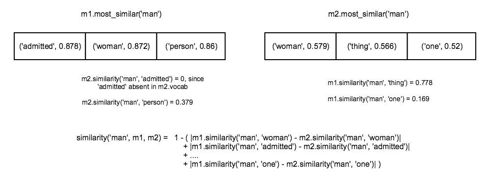
   • Find the topn_similar most similar words to w for both models (I used a value of 10), and create vectors topn_similar_m1 and topn_similar_m2 containing their similarity scores, if w is missing in either model, take a vector of zeroes of size topn_similar for that model
   • Find the difference between topn_similar_m1 and topn_similar_m2, if a word is present in the vocab for both models, but present in only one of topn_similar_m1 and topn_similar_m2, use its similarity to w as the score, if a word is missing in the vocab for either model, use 0 as its similarity score, while computing the difference
   • Sum up these differences and normalize the result to get a dissimilarity measure for word w in the two models
3. Sum up all dissimilarity scores and normalize to get a dissimilarity score for the two models

The metric obtained is independent of the actual word vectors learned for the words, and instead takes into account the difference in contexts the word appears in in the two models.

Getting to the implementation, I used gensim to train and work with word vectors. It takes in as input an array of sentences constituting a document, and trains a set of word vectors. The model exposes a method to calculate the n most similar words to a given word. So, a naive implementation of the method to calculate the dissimilarity metric looks something like -

def model_dissimilarity_basic(m1, m2, num_chosen_words=100, topn=10):
  dissimilarity = 0.0

  # Sampling from models individuals to eliminate a document with a larger vocab dominating the sampling process
  m1_words = random.sample(m1.vocab.keys(), num_chosen_words/2)
  m2_words = random.sample(m2.vocab.keys(), num_chosen_words/2)
  for i in range(num_chosen_words/2):
    word_dissimilarity_score = word_dissimilarity(m1_words[i], m1, m2, topn)
    dissimilarity += word_dissimilarity_score

    word_dissimilarity_score = word_dissimilarity(m2_words[i], m2, m1, topn)
    dissimilarity += word_dissimilarity_score

  dissimilarity /= num_chosen_words
  return dissimilarity

def word_dissimilarity(given_word, given_model, target_model, topn = 10):
  # given_model.most_similar('man') => [(u'woman', 0.8720022439956665), (u'person', 0.8601664304733276)...]
  given_similar_words = {obj[0]:obj[1] for obj in given_model.most_similar(given_word, topn=topn)}
  dissimilarity = 0.0

  if not given_word in target_model:
    dissimilarity += sum(given_similar_words.values())/topn
  else:
    target_similar_words = {obj[0]:obj[1] for obj in target_model.most_similar(given_word, topn=topn)}
    union_similar_words = set(given_similar_words.keys()) | set(target_similar_words.keys())
    for word in union_similar_words:
      if word in given_similar_words:
        similarity_given_model = given_similar_words[word]
      elif word in given_model.vocab:
        similarity_given_model = given_model.similarity(given_word, word)
      else:
        similarity_given_model = 0

      if word in target_similar_words:
        similarity_target_model = target_similar_words[word]
      elif word in target_model.vocab:
        similarity_target_model = target_model.similarity(given_word, word)
      else:
        similarity_target_model = 0
      dissimilarity  += abs(similarity_given_model - similarity_target_model)
    dissimilarity /= len(union_similar_words)
  return dissimilarity

This turns out to be quite slow. Understanding why requires a slightly more detailed explanation of how the most_similar method in gensim works. Gensim stores a word-index mapping in self.vocab and the actual word vectors in self.syn0 (self.syn0norm for the normalized vectors). A call to model.most_similar(word) simply does this -

1. Look up the word vector for the given word
2. Multiply it with self.syn0, getting a vector of similarity scores
3. Take the topn highest scores from the resulting vector of scores, and maps the corresponding indices to actual words

The entire process is repeated for each word in the sampled words.

The two slowest steps here are the matrix multiplication ( O(N^2 * V), N: word vector size, V: vocabulary length) needed to compute the cosine similarities, and the partial sort ( O(V) V: vocabulary length) to calculate the topn scores from the entire vector of scores. Both these calculations grow linearly with V, the vocabulary size for the model. N is usually not a very large number (100-300), and the same value is used, so more or less, both these calculations are linear with size of vocabulary.

These calculations are performed once for calculating topn similar words for every single sampled word. Suppose we sample S words to calculate similarity between the two models, an additional factor of S comes into the picture. Here is where the optimization comes in:

np.matmul works in such a manner, that a single, large matrix multiplication (for calculating similarity scores for all S x V word pairs) takes significantly less time than calculating similarity scores for each word in S individually. Hence, I implemented a vectorized version of the algorithm described above, where I calculate similarity scores for the sampled words with respect to the model vocabulary in a single matrix multiplication. I ran a simple profiling of both methods over 50 iterations, computing similarity between two models (vocabulary sizes 15073 and 17011) for topn = 2000 , and the total times are shown below:

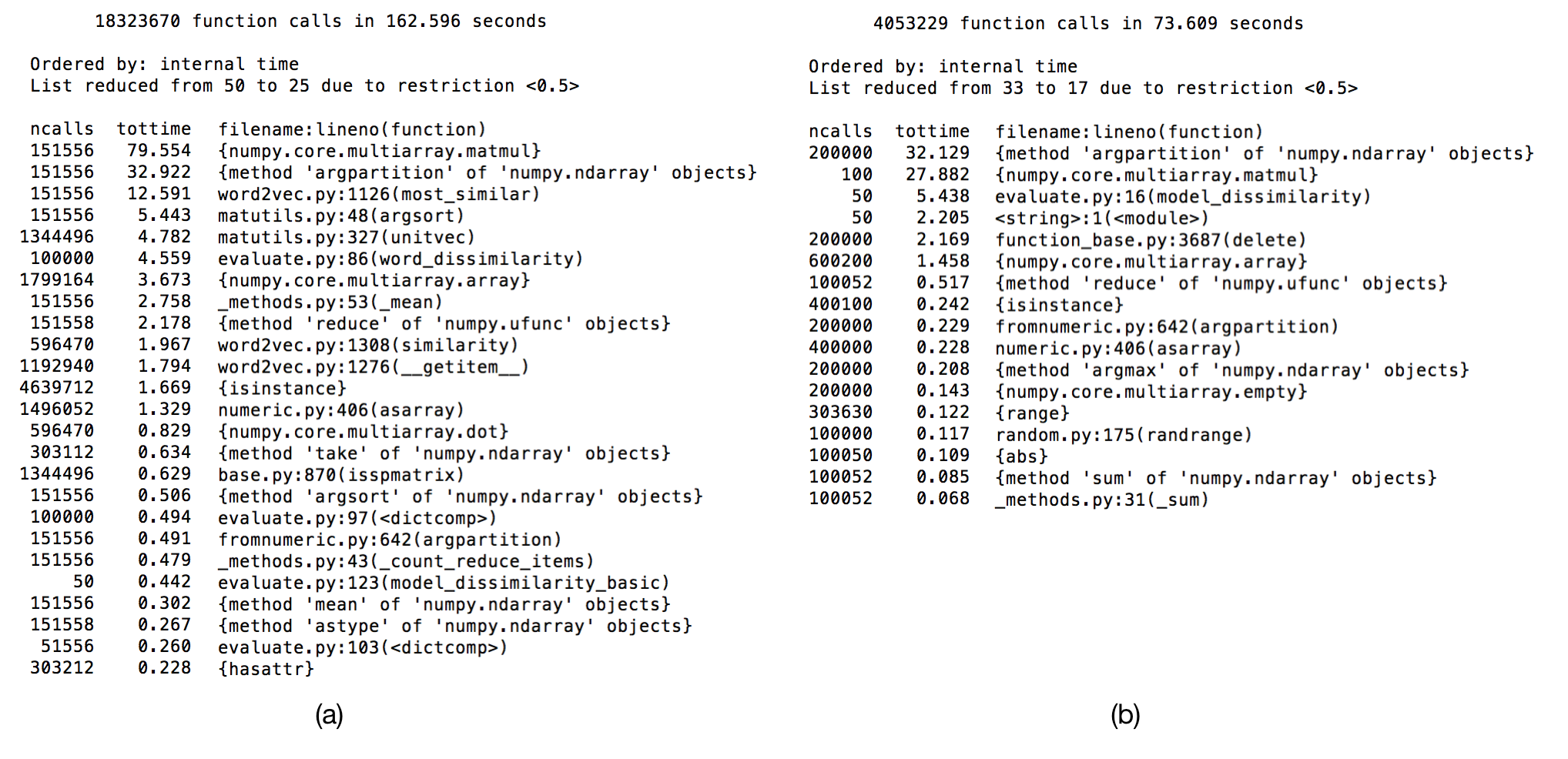
We see that np.matmul (numpy.core.multiarray.matmul) takes almost thrice the time in the first case (79.554s) than in the second (27.882s). The number of times np.matmul is being called is also very different - it is called twice in each iteration for the vectorized method, and an average of ~3k times per iteration for the naive method. Of course, the size of the matrices being multiplied is very different - the vectorized approach involves two multiplications of matrices with dimensions V x N and N x topn, the gensim approach around 3k multiplications of matrices with dimensions V x N and N x 1.

The vectorized approach actually involves a higher number of computations - this is because in the naive method, model.most_similar is only called in case the word is present in the model, hence avoiding a few multiplications. However, despite the higher number of computations, numpy seems to perform a large matrix multiplication much faster than a large number of smaller matrix multiplications. This seems like another interesting tidbit to find out more about, and I might look into this later. On a related note, np.argpartition (method for partially sorting an array, taking a significant chunk of time) seems to work the other way round - running it on a single large matrix took significantly more time than running it on the individual rows of the matrix.

The code for the vectorized method can be found here.

Getting back to the problem at hand, once I had a similarity measure between documents, clustering them seemed like the obvious next step. The only issue was, word2vec works better for larger document sizes, and most clustering datasets that I could quantitatively evaluate my method on seemed to have fairly small document sizes. So I simply downloaded a sample from the top 100 ebooks on Project Gutenberg and ran it on those - I was quite interested in seeing how classic literature could be clustered. I used Spectral Clustering for clustering the books from the similarity matrix, and Spectral Embedding, a manifold learning technique to reduce the dimensionality to 2 dimensions for visualization.

Results

There are a few anomalies, but on the whole the results seemed fairly interesting. Arthur Conan Doyle and Jane Austen get entire clusters of their own. The “yellow” cluster seems to contain books mostly in the young adult adventure genre (Mark Twain, Three Men in a Boat, Treasure Island) with Ulysses being a complete exception. The “blue” cluster has all the epics (Les Miserables, War and Peace, Crime and Punishment, Monte Cristo), and Tolstoy and Dostoyevsky are both Russian greats of the same era, with similar styles and influences.

The fourth cluster contains mostly non-fiction, and a lot of them are about politics, governance and society (Wealth of Nations, The Republic, Utopia, Leviathan, John Locke, Machiavelli). The sixth cluster has only plays, the seventh groups together Charles Dickens and the Bronte sisters, with Oscar Wilde and Agatha Christie being out of place.

The red cluster is a little more diverse, having some sci-fi/fantasy novels (Wizard of Oz, H.G Wells, Lewis Caroll, Peter Pan), but also Around the World in Eighty Days and Agatha Christie. The orange cluster consists of epic poems, (Paradise Lost, The Divine Comedy, Iliad, William Blake), The Bible, Shakespeare, with Don Quixote and Common Sense again anomalies.

Edgar Allen Poe and Marh Shelley both wrote morbid stories with dark themes and appear together in the last cluster, which also contains Walden, Moby Dick and The Scarlet Letter - no common threads there.

A small note on preprocessing - the whole analysis above has been performed with absolutely no preprocessing of the text, except for removing the Project Gutenberg header and footer. I’m curious to see how steps like stopword removal, removing punctuation, lemmatization or simply downcasing the entire text would affect the process. Analyzing this properly would require that I first have a way of quantitatively measuring the performance of the document clustering algorithm I’ve described, which isn’t possible with the Project Gutenberg dataset. There was a noticeable improvement in the accuracy for the semantic association task provided with the gensim Word2Vec class when I downcased all the text before training, but that is hardly conclusive. Open to hearing your ideas about this.

I’m also interested in seeing how this approach compares with traditional statistical approaches like tf-idf, LSA (Latent Semantic Analysis), LDA etc. Theoretically, word2vec takes into account more information - tf/idf has no notion of word similarity or meaning, while the word2vec representation considers semantic information. Of course, the representation actually learnt may or may not be accurate, so it’d be interesting to quantitatively compare the two approaches.